Saving Your PowerPoint Presentation

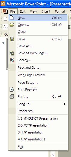
To save your PowerPoint presentation use one of the following commands.

Press  Ctrl+S

File _ Save

Click  Save     Button in the Standard Toolbar

Creating a Presentation

Blank Presentation

You can use this to create a new, blank presentation using the default settings for text and colors.

From Design Template

Use this to create a new presentation based on one of the PowerPoint design templates.

From Auto Content Wizard

You can use Auto Content Wizard to create a new presentation by prompting you for information about content, purpose, style, handouts, and output. The new presentation contains sample text that you can replace with your own information.

Choose  presentation

You can use this option to open an existing presentation in your Floppy Disk, Hard Disk or any other location  so that you can edit or show it.

Creating a Presentation

When PowerPoint stars, it presents you with a variety of options for creating or opening presentations. Click File - New
or
Click File - New - Blank Presentation - Apply Slide Layouts

The Standard Power Point Window

Starting Microsoft PowerPoint

To start Microsoft PowerPoint, use one of the following commands 

	i.	Click Start -- All Programs -- Microsoft PowerPoint
	ii.	Double Click on PowerPoint Icon in the Desktop

Microsoft Power Point XP

         Microsoft PowerPoint is the presentation Software which comes with MS Office. This presentation graphics program helps you create simple, professional and attractive presentations.

Adding A Custom List

The Custom Lists option allows you to add a New List to your Custom Lists Box The advantage of this is that you needn’t to retype a list which you are frequently using.

	i.	To add a New Custom list Select Tools - Options - Custom Lists
	ii.	Click New List in the Custom lists box to create a new list, and then type the entries in the List entries box. The first character cannot be a number. Press Enter Key to  separate each entry or type the list separating by comas. .( Ex: Officer Training Wing , Navigation School, Gunnery School, Commutation School, Edp School, Supply School, Electrical School, Combat Training School, ASW School)
	iii.	Then, Click Add Button to add your New List to List Entries Box and finally click Ok

Conditional Formatting

You can use Conditional Formatting to apply formats to selected cells that meet specific criteria based on values or formulas you specify.

	a.	First select the Cells or Range Of Cells that you want to apply Conditional Format and then Select Format - Conditional Formatting
	b.	Then click the operator you want to use to set the condition on the selected cell range (Ex : Cell Value is Less than or Equal to 5000)
	c.	Select the format elements you want to apply with conditional formatting. You can apply only one conditional format to a cell at a time.
	d.	After giving all the conditions and formats Click Ok Note : You can give maximum three Conditional Formats to a Selected Cell Range

Data Validation

You can use Data validation to define what data is valid for individual cells or cell ranges; restricts the data entry to a particular type, such as whole numbers, decimal numbers, or text; and sets limits on the valid entries.

	a.	First select the Cells or Cell Range to validate and go to Data - Validation
	b.	Then type the Validation Criteria , Input Message and Error Alert (Style ,Title and Message) and finally click Ok

About Charts in Ms Excel

Charts are visually attractive and make it easy for users to see comparisons, patterns, and trends in data. For most 2-D charts, you can change the chart type of either a data series or the entire chart. For bubble charts, you can change only the type of the entire chart. For most 3-D charts, changing the chart type affects the entire chart. For 3-D bar and column charts, you can change a data series to the cone, cylinder, or pyramid chart type.

Creating a Chart Using Chart Wizard on Selected Data

City	Minimum	Maximum
Ratnapura	18	30
Colombo	20	26
Kandy	16	21
Badulla	19	29
Galle	17	27
Trincomalee	25	31

	a.	First select Cell Range that Contain data with Column Headings
	b.	Select Insert - Chart
	c.	Next you will be prompted to Chart Wizard Dialog Box , From Chart Wizard Dialog Box Select Standard Types Tab and then select Column Chart Type and 3-D Visual Effect and finally Click Next Button.
	d.	Click Next Button in next step also
	e.	In the next step type following in required Text boxes and Click Next Button Chart Title : Normal Temperature Of Six Cities In Sri Lanka on March 2003 Category (X) axis : Cities Value (Z) axis : Temperature In Celsius
	f.	Finally Click Finish Button

Functions in Excel

i. UPPER

The upper function is used to convert a text into uppercase. =Upper (“trincomalee”) will give you TRINCOMALEE

ii. LOWER

Converts all uppercase letters in a text string to lowercase. =Lower (“CHINTHAKA”) will give you chinthaka

iii. PROPER

Capitalizes the first letter in a text string and any other letters in text that follow any character other than a letter. Converts all other letters to lowercase letters. =Proper (“online it academy”) will give you Online It Academy

iv. TRIM

Removes the unnecessary spaces from a string =Trim (“Online It Academy”) → Online It Academy

v. REPT

Repeat a text a given number of times. =REPT (“@ # %”, 20)

vi. SQRT

Returns a positive square root. = sqrt (81) → 9

vii. ROUND

Rounds a number to a specified number of digits. =Round (2.5678,2) → 2.57

viii. POWER

Returns the result of a number raised to a power. = Power (7,3) → 343

ix. MOD

Returns the remainder after a number is divided by another number. = mod(17,6) → 5

x. INT

Returns the integer value after a number is divided by another number. =Int(10/3) → 3

xi. POWER

Returns the result of a number raised to a power. =Power(5,3) → 125

xii. SUM

Adds all the numbers in a range of cells. = Sum(12,5,7) → 24 = Sum (A1 : A5)

xiii. AVERAGE

Returns the average (arithmetic mean) of the arguments. = Avg (3,4,5) → 4 = Average (A1: A5)

xiv. MAX

Returns the largest value in a set of values. = Max (12,45,6,67,82,11) → 82 = Max (A1: A5)

xv. MIN

Returns the smallest value in a set of values. = Max (12,45,6,67,82,11) → 6 = Max (A1: A5

Using Functions in Ms Excel

Functions are predefined formulas that perform calculations by using specific values, called arguments, in a particular order, or structure. Functions can be used to perform simple or complex calculations.

a. The structure of a function

The structure of a function begins with an equal sign (=), followed by the function name, an opening parenthesis, the arguments for the function separated by commas, and a closing parenthesis.

b. Function name.

For a list of available functions, click a cell and press SHIFT+F3

c. Arguments.

Arguments can be numbers, text, logical values such as TRUE or FALSE.

d. Argument tool tip.

A tool tip with the syntax and arguments appears when you type the function. For example, type =ROUND (and the tool tip appears. Tool tips appear only for built-in functions..

e. Create a Formula

The formulas perform calculations on values in your worksheet. A formula starts with an equal sign (=). For example, the following formula multiplies 2 by 3 and then adds 5 to the result. =5+2*3

The Border Tab

Border

Click a line style in the Style box, and then click the buttons under Presets or Border to apply borders to the selected cells. To remove all borders, click the None button. You can also click areas in the text box to add or remove borders.

Line style

Select an option under Style to specify the line size and style for a border. If you want to change a line style on a border that already exists, select the line style option you want, and then click the area of the border in the Border model where you want the new line style to appear.

Color

Select a color from the list to change the Border color

The Font Tab

The font tab will allow you to select Font Type, Font Style, Font Color, Font Size and Underline Type

The Alignment Tab

The Alignment Tab allows you to adjust Text alignment, Text control and Orientation

Horizontal

Select an option in the Horizontal list box to change the horizontal alignment of cell contents. By default, Microsoft Excel aligns text to the left, numbers to the right. The default horizontal alignment is General. Changing the alignment of data does not change the data type.

Vertical

Select an option in the Vertical box to change the vertical alignment of cell contents. By default, Microsoft Excel aligns text vertically on the bottom of a cell. The default horizontal alignment is General

Orientation

Sets the amount of text rotation in the selected cell. Use a positive number in the Degree box to rotate the selected text from lower left to upper right in the cell. Use negative degrees to rotate text from upper left to lower right in the selected cell.

Wraps text

Wraps text into multiple lines in a cell.

Shrink to fit

Reduces the visible size of font characters so that all data in a selected cell fits within the column. The character size is adjusted automatically if you change the column width.

Merge Cells

Combines two or more selected cells into a single cell. The cell reference for a merged cell is the upper-left cell in the original selected range.

The Number Tab

The Number Tab allows you to change the number format. Click an option in the Category box, and then select the options that you want to specify a number format. The Sample Box shows how selected cells will look with the formatting you choose.

Format Cells

You can use Format Cells Dialog Box to apply formats to the selected cells. To format a cell or selected cells, Go to Format --Cells or Press Ctrl + 1.

Freeze Panes

Use the Freeze Panes to keep column or row titles in view while you're scrolling through a worksheet. Freezing titles on a worksheet does not affect printing.

Protecting your Worksheet

You can use Protect sheet option to protect entire worksheet or selected cells.
To protect entire worksheet select Tools - Protection - Protect sheet
To Protect selected cells, follow the steps given below

	a.	Select the entire worksheet and then, Go to Format - Cells - Protection and uncheck the locked Check Box and then Click Ok Button.
	b.	Next, Select the Cell Range that you want to Protect and then ,Go to Format - Cells - Protection check the locked Check Box and then Click Ok Button.
	c.	Finally ,Select Tools - Protection - Protect sheet

Note : If you want to unprotect the sheet , Select Tools - Protection - Unprotect sheet.

Setting up your Paper Size and Margins

The Page Setup option allows you to set your Paper Size, Margins and Orientation and other layout options for the active file, to select this option go to File - Page Setup

		Setting up paper margins

Moving and Coping Data

To move Data

	i.	First select the Cell Range that contain data and then Go to Edit - Cut or Press Ctrl + X
	ii.	Place the cursor where you want to move data and the Go to Edit - Paste or Press Ctrl + V

Note: To simply move data, First select the Cell Range that contain data and then drag the Cell Range to required place and finally release the mouse button.

To copy Data

	i.	First select the Cell Range that contain data and then Go to Edit - Copy or Press Ctrl + C
	ii.	Place the cursor where you want to copy data and the Go to Edit - Paste or Press Ctrl + V

Note: To simply copy data, First select the Cell Range that contain data and then drag the Cell Range to required place by pressing Ctrl Key and finally release the mouse button.

Renaming and Deleting A Worksheet

Renaming A Worksheet

	i.	To rename a worksheet Double Click on the Worksheet Tab
	ii.	Delete existing name and Type a New Name
	ii.	Finally Press Enter Key or Click anywhere in Worksheet

Deleting Worksheets

	i.	To delete a Worksheet Right Click on Worksheet Tab and then select Delete.
	ii.	To delete multiple worksheets, Select the required worksheets while pressing Shift Key and then ,Select Edit - Delete Sheet

Inserting a new Worksheet

	a.	To insert a single worksheet
	i.	Click Worksheet on the Insert menu.
	b.	To insert multiple worksheets.
	i.	Determine the number or worksheets you want to insert.
	ii.	Hold down Shift Key, and then select the number of existing worksheet tabs that you want to insert in the open workbook.

Example: If you want to insert three new worksheets, select three existing worksheet tabs and then click Worksheet on the Insert menu.
Note: You can insert maximum 255 Worksheets in a Workbook.

Selecting Data or Cells

	i.	Text in a Cell : Double-click in the cell, and then select the text in the cell.
	ii.	A Single Cell : Click the cell, or press the arrow keys to move to the cell.
	iii.	A Range Of Cells : Click the first cell of the range, and then drag to the last cell
	iv.	A Large Range Of Cells : Click the first cell in the range, and then hold down Shift Key and click the last cell in the range. You can scroll to make the last cell visible.
	v.	All Cells on A Worksheet : Click the Select All button.
	vi.	Nonadjacent Cells Or Cell Ranges : Select the first cell or range of cells, and then hold down Ctrl and select the other cells or ranges.
	vii.	An Entire Row Or Column : Click the row or column heading.
	viii.	Adjacent Rows Or Columns : Drag across the row or column headings. Or select the first row or column; then hold down Shift and select the last row or column.
	ix.	Nonadjacent Rows Or Columns : Select the first row or column, and then hold down Ctrl and select the other rows or columns.
	x.	Cancel A Selection Of Cells: Click any cell on the worksheet.

Inserting Blank Cells, Rows, or Columns

i. To insert Blank cells, Rows, or Columns do one of the following:

	a.	To insert new blank Cells: Select the number of cells as you want to insert
	b.	To insert a single Row : Click a cell in the row immediately below where you want the new row. For example, to insert a new row above row 5, click a cell in row 5.
	c.	To Insert multiple Rows : Select number of rows that you want
	d.	To Insert a single Column: Click a cell in the column immediately to the right of where you want to insert the new column. For example, to insert a new column to the left of column B, click a cell in column B.
	e.	To Insert multiple Columns : Select the number of columns you want .

ii. On the Insert menu, Click Cells, Rows, or Columns.

Deleting Cells, Rows, or Columns

	i.	Select the Cells, Rows, or Columns that you want to delete.
	ii.	On the Edit menu, click Delete.

Note: If you are deleting a range of cells, click Shift cells left, Shift cells up, Entire row, or Entire column in the Delete dialog box.

Closing and Exit from Ms Excel

                Closing a Work Book

To close your Active Work Book select File  Close from Main Menu or Press Ctrl + F4 simultaneously.

                To exit from Microsoft Excel

To exit  from  Microsoft Excel , Select  File  Exit  from Main Menu or press Alt + F4  at the same time.

Opening an Excel Workbook

To open an Excel Workbook use one of the following commands

	a.	File  Open
	b.	In Open Dialog Box select the file that you want to open and click Open Button or simply double click on the file.

Saving an Excel Workbook

To save an Excel Workbook

	i.	File  Save.
	ii.	Select the location where you want to save the workbook and give a desired name and finally click Save button.
		Note : If you want to give a Password to your Excel Workbook, go to Tools  Security Options before you save your Workbook.

Insert and Hiding Toolbars

To Insert or hide a toolbar do one of the following

	i.	Right-click on any toolbar and then click the toolbar you want to display or hide on the Popup menu.
	ii.	View --- Toolbar in the Main Menu and then select or deselect toolbars that you want.

The Standard Excel Window

Starting Microsoft Excel XP

To start Microsoft Excel use one of the following commands 

	i.	Click Start  -- All Programs  -- Microsoft Excel
	ii.	Double Click On Excel icon in Desktop

Software & Hardware Requirements for MS Excel XP

	i.	Operating Systems :	Windows 98 Second Edition, Windows Me ,Windows 2000 or Windows XP
	ii.	Processor Speed   :	Minimum 500 MHz
	iii.	RAM                    :	Minimum 64 MB RAM

Ms Excel XP

Excel is a spreadsheet program. Spreadsheets allow easy entering and maintenance of data. Companies often prepare budgets and reports and maintain a large amount of data pertaining to its business. Excel can be used to maintain financial statistics, reports, balance sheets etc. It offers features for quick creation of these statements. Besides offering the features to maintain data, it also offers methods for performing calculations quickly and efficiently and ways to analyze data create consolidated reports and for creating charts to attractively present your data.

Adjusting Margins: Ruler Option

             The margins are located on the Ruler at the top of the screen, on the left and on the right where the gray and white areas meet.

a.		If the Ruler is not displayed, from the View menu, select Ruler
b.		From the View menu, select Print Layout
c.		Move your cursor to the ruler line and position it over the margin you wish to change The cursor will take the shape of a double-headed arrow.
d.		Hold down your mouse button and drag the margin to the desired width ,in Windows to see the margin measurements, hold down the [Alt] key while dragging the margin.